stat_QC_Capability()
Kenith Grey
2018-12-04
Description
ggplot stat function for QC capability anaylsis. Function renders lines, lables and summary statistics. Works best with histogram and density plots.
Usage
stat_QC_Capability(LSL, USL, method = "xBar.rBar",
show.lines = c("LSL", "USL"), line.direction = "v",
show.line.labels = TRUE, line.label.size = 3,
show.cap.summary = c("Cp", "Cpk", "Pp", "Ppk"), cap.summary.size = 4,
px = Inf, py = -Inf, digits = 3)
Specialized Args: Stat_QC()
- LSL: numeric, Customer’s lower specification limit
- USL: numeric, Customer’s Upper specification limit
- method: string, calling the following methods:
- Individuals Charts: XmR,
- Studentized Charts: xBar.rBar, xBar.rMedian, xBar.sBar, xMedian.rBar, xMedian.rMedian
- show.lines: vector, indicating which lines to draw ie., c(“LCL”, “LSL”, “X”, “USL”, “UCL”)
- LCL: Lower Control Limit
- LSL: Lower Specification Limit
- X: Process Center
- USL: Upper Specification Limit
- UCL: Upper Control Limit
- line.direction: string “v” or “h”, specifies which direction to draw lines.
- show.line.labels: boolean, if TRUE then draw.
- line.label.size: numeric, control the size of the line labels.
- show.cap.summary: vector, indicating which lines to draw ie., c(“TOL”,“DNS”, “Cp”, “Cpk”, “Pp”, “Ppk”, “LCL”, “X”, “UCL”, “Sig”). The order given in the vector is the order presented in the graph.
- TOL: Tolerance in Sigma Units (USL-LSL)/sigma
- DNS: Distance to Nearest Specification Limit in Simga Units
- Cp: Cp (Within)
- Cpk: Cpk (Within)
- Pp: Pp (Between)
- Ppk: Ppk (Between)
- LCL: Lower Control Limit
- X: Process Center
- UCL: Upper Control Limit
- Sig: Sigma from control charts
- cap.summary.size: numeric, control the size/scale of the summary text box.
- px: numeric, x position for summary text box. Use Inf to force label to x-limit.
- py: numeric, y position for summary text box. Use Inf to force label to y-limits. May also need vjust parameter.
- digits: integer, how many digits to report.
Value
QC capability layer for histogram and density plots.
See Also
for more control over lines, labels, and capability data see the following functions:
stat_QC_cap_vlabels
stat_QC_cap_hlabels
stat_QC_cap_vlines
stat_QC_cap_hlines
stat_QC_cap_summary
Examples
# Load Libraries ----------------------------------------------------------
require(ggQC)
require(ggplot2)
# Setup Data --------------------------------------------------------------
set.seed(5555)
Process1 <- data.frame(ProcessID = as.factor(rep(1,100)),
                      Value = rnorm(100,10,1),
                      Subgroup = rep(1:20, each=5),
                      Process_run_id = 1:100)
set.seed(5556)
Process2 <- data.frame(ProcessID = as.factor(rep(2,100)),
                      Value = rnorm(100,20, 1),
                      Subgroup = rep(1:10, each=10),
                      Process_run_id = 101:200)
df <- rbind(Process1, Process2)
Histogram and Density-Base Plots
Depending on your scale, you’ll need to leave a bit of room to the left or right of your histogram for the capability statistics if you choose to present them. To provide the necessary space, use
scale_x_continuous(expand = expand_scale(mult = c(0.15,1.3)))
XmR_Cap_Hist <-  ggplot(df[df$ProcessID == 1,], aes(x=Value, QC.Subgroup=Subgroup)) +
geom_histogram(binwidth = 1, color="purple") +
 geom_hline(yintercept=0, color="grey") +
 scale_x_continuous(expand =  expand_scale(mult = c(0.15,1.3))) +
 ylim(0,45) +
 ggtitle("Histrogram Capability", subtitle = "Base Graph")

XmR_Cap_dens <- ggplot(df[df$ProcessID == 1,], aes(x=Value, QC.Subgroup=Subgroup)) +
geom_density(bw = .4, fill="purple", trim=TRUE) +
 geom_hline(yintercept=0, color="grey") +
 scale_x_continuous(expand =  expand_scale(mult = c(0.15,1.3)))  + ylim(0,.5) +
ggtitle("Denisty Capability", subtitle = "Base Graph")

gridExtra::grid.arrange(XmR_Cap_Hist, XmR_Cap_dens, nrow=1)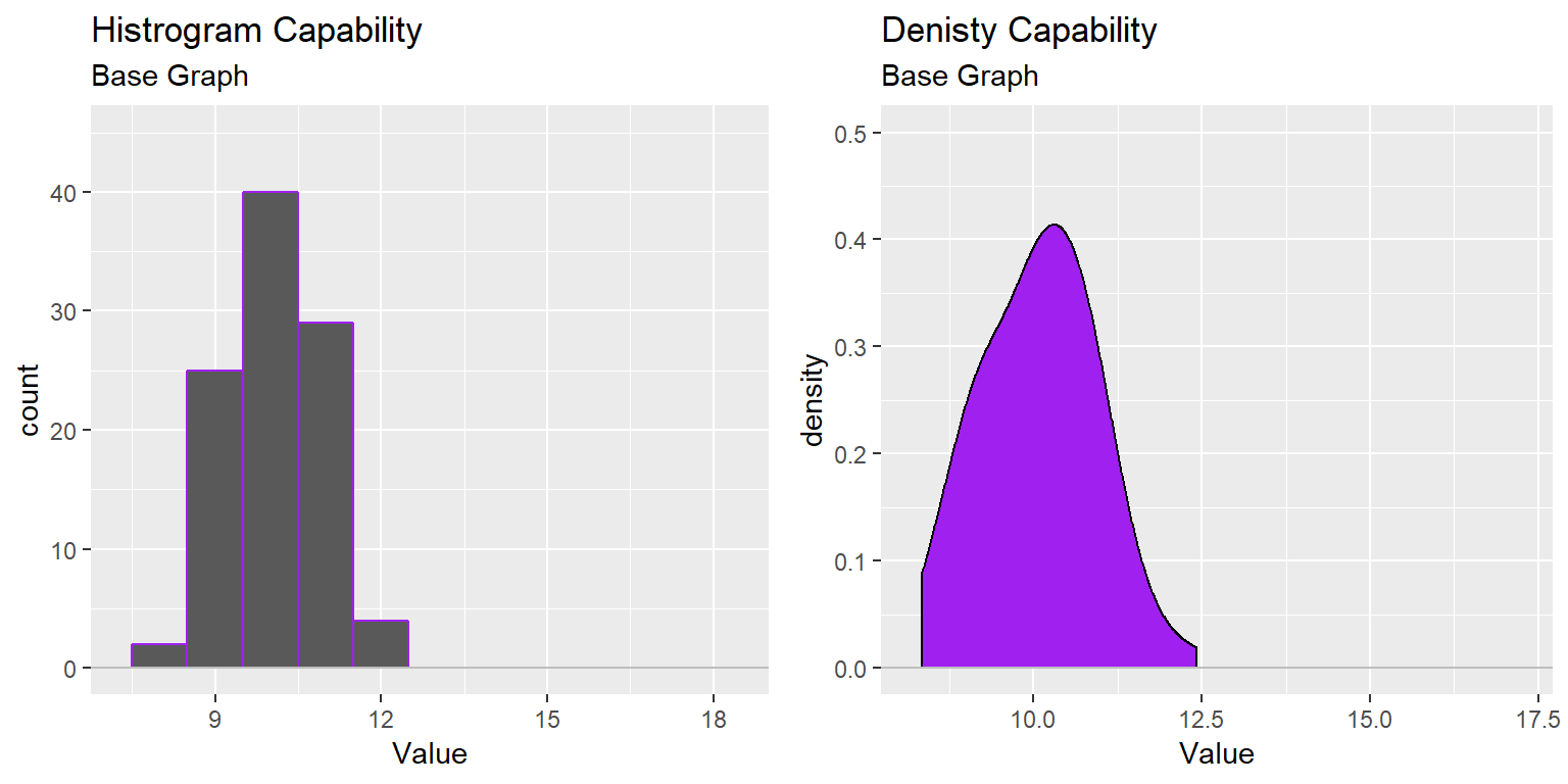
Basic Capability Lines and Stats
XmR_Cap_Hist2 <- XmR_Cap_Hist +
 stat_QC_Capability(LSL=5, USL=15, show.cap.summary = "all", method="XmR") +
 ggtitle("Histrogram Capability", subtitle = "Showing Complete Capabiltiy Summary")

XmR_Cap_dens2 <- XmR_Cap_dens +
 stat_QC_Capability(LSL=5, USL=15,
                    show.cap.summary = c("Cp", "Cpk"),
                    method="XmR") +
ggtitle("Denisty Capability", subtitle = "Showing Cp ane Cpk Capabiltiy Summary")

gridExtra::grid.arrange(XmR_Cap_Hist2, XmR_Cap_dens2, nrow=1)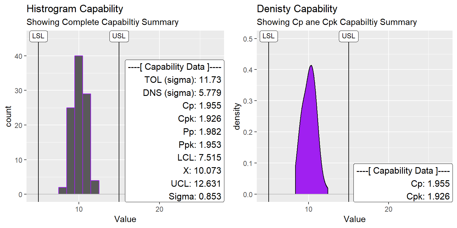
Change Number of Digits
XmR_Cap_Hist2 <- XmR_Cap_Hist +
 stat_QC_Capability(LSL=5, USL=15, show.cap.summary = "all",
                    method="XmR", digits = 1) +
 ggtitle("Histrogram Capability", subtitle = "digits = 1")

XmR_Cap_dens2 <- XmR_Cap_dens +
 stat_QC_Capability(LSL=5, USL=15,
                    show.cap.summary = c("Cp", "Cpk"),
                    method="XmR", digits=4) +
ggtitle("Denisty Capability", subtitle = "digits = 4")

gridExtra::grid.arrange(XmR_Cap_Hist2, XmR_Cap_dens2, nrow=1)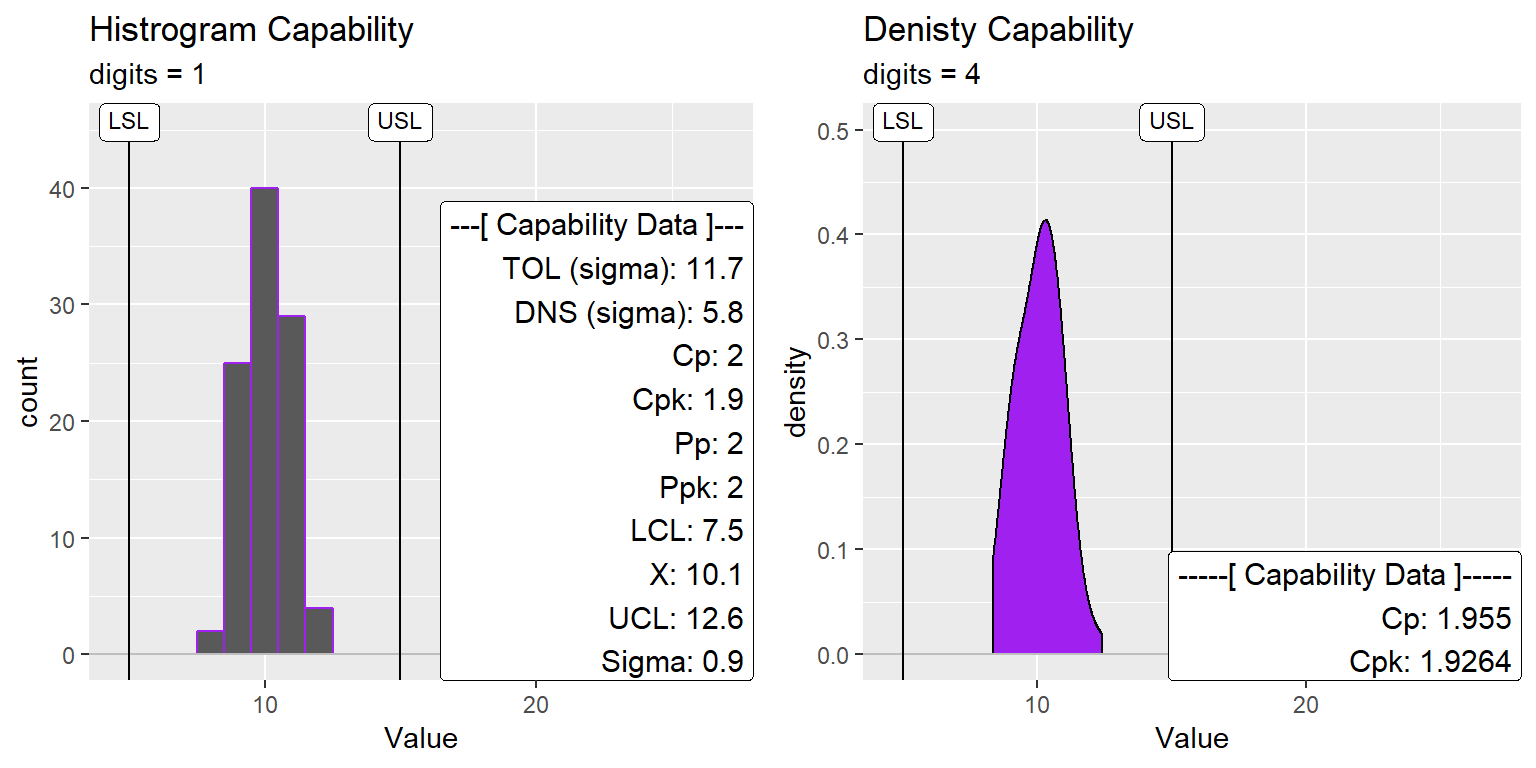
Change Lines Drawn
XmR_Cap_Hist2 <- XmR_Cap_Hist +
 stat_QC_Capability(LSL=5, USL=15, show.cap.summary = "all",
                    method="XmR", digits = 1,
                    show.lines = c("LSL","LCL","X","UCL", "USL")
                      ) +
 ggtitle("Histrogram Capability", subtitle = "show.lines = c('LSL','LCL','X','UCL', 'USL')")

XmR_Cap_dens2 <- XmR_Cap_dens +
 stat_QC_Capability(LSL=5, USL=15,
                    show.cap.summary = c("Cp", "Cpk"),
                    method="XmR", digits=4,
                    show.lines = c("LSL","X","USL")
                    ) +
ggtitle("Denisty Capability", subtitle = "show.lines = c('LSL','X','USL')")

gridExtra::grid.arrange(XmR_Cap_Hist2, XmR_Cap_dens2, nrow=1)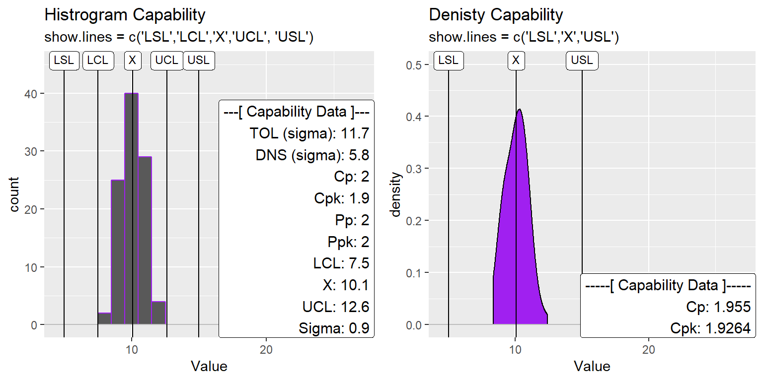
Change Capability Data Size
XmR_Cap_Hist2 <- XmR_Cap_Hist +
 stat_QC_Capability(LSL=5, USL=15, show.cap.summary = "all",
                    method="XmR", digits = 1,
                    show.lines = c("LSL","LCL","X","UCL", "USL"),
                    cap.summary.size = 3
                    ) +
 ggtitle("Histrogram Capability", subtitle = "cap.summary.size = 3")

XmR_Cap_dens2 <- XmR_Cap_dens +
 stat_QC_Capability(LSL=5, USL=15,
                    show.cap.summary = c("Cp", "Cpk"),
                    method="XmR", digits=4,
                    show.lines = c("LSL","X","USL"),
                    cap.summary.size =  2
                    ) +
ggtitle("Denisty Capability", subtitle = "cap.summary.size = 2")

gridExtra::grid.arrange(XmR_Cap_Hist2, XmR_Cap_dens2, nrow=1)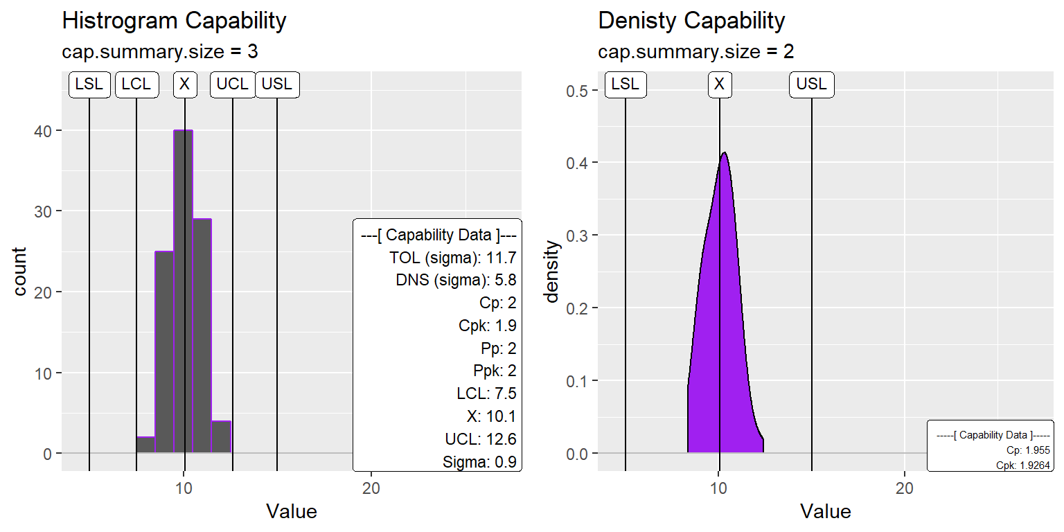
xBar.rBar or xBar.sBar Capability
All the capabilites discussed above will work with plots calculated from xBar.rBar or xBar.sBar statistics. The difference is QC.Subgroup must be specified in aes() portion of the ggplot initialization. Here is an example.
#Look closely in the aes statement.
ggplot(df[df$ProcessID==1,], aes(x=Value, QC.Subgroup=Subgroup)) +
 geom_histogram(binwidth = 1) +
 stat_QC_Capability(LSL=5, USL=15, method="xBar.rBar") +
 scale_x_continuous(expand =  ggplot2::expand_scale(mult = c(0.15,.8))) #+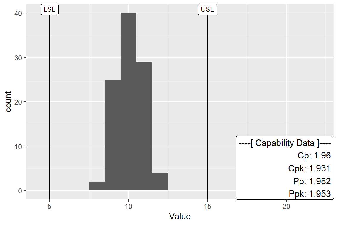
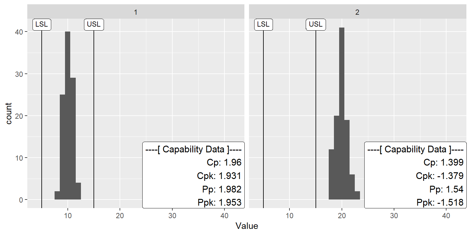
A Faceting Example
ggplot(df, aes(x=Value, QC.Subgroup=Subgroup)) +
 geom_histogram(binwidth = 1) +
 stat_QC_Capability(LSL=5, USL=15, method="xBar.rBar") +
 scale_x_continuous(expand =  ggplot2::expand_scale(mult = c(0.15,1.1))) +
 facet_wrap(~ProcessID, nrow=1)